
下载
© 2011 Microchip Technology Inc. DS01415A-page 1
AN1415
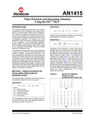
INTRODUCTION
The required bandwidth for data access from off-chip
components can be a bottleneck in the system perfor
-
mance for microcontroller (MCU) video applications.
This restriction translates into limiting the number of
read and write accesses to the external memory device
during a given time period. A popular solution is to use
a compression algorithm. The quality of the video
depends on, and in most cases, is directly proportional
to the complexity of the compression algorithm.
Another solution is to adhere to the bandwidth limita
-
tions by reading a lower resolution video and to rescale
it (i.e., upscaling) during display. There are several
methods of upscaling a video.
This application note describes four methods of playing
a video file using a PIC
®
microcontroller (MCU) and
hardware solutions available from Microchip. Two
major constraints for these solutions are the bandwidth
required for the data access and the processor speed.
For example, the first method uses video upscaling to
achieve the desired performance, while the second
method takes advantage of the LCD controller on the
Multimedia Expansion Board (MEB) to write the video
data directly to the frame buffer. Both of these methods
read a video file from a Secure Digital (SD) card and
display it on a QVGA LCD screen.
METHOD 1: VIDEO PLAYBACK ON
PIC32 USING UPSCALING BY
INTERPOLATION
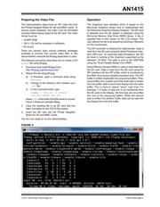
The data throughput required to play the video file can
be calculated using the formula in
Equation 1.
EQUATION 1:
For uncompressed QVGA video at 30 frames per sec-
ond and 16 bits per pixel, the bandwidth required is
calculated, as shown in
Equation 2.
EQUATION 2:
Using the linear interpolation technique, we can reduce
this requirement, as shown in
Equation 3.
EQUATION 3:
Interpolation is the technique of using known data to
estimate values of unknown data. The known data is
the data with smaller resolution. The unknown data is
the difference in the data between the smaller and the
higher resolution images.
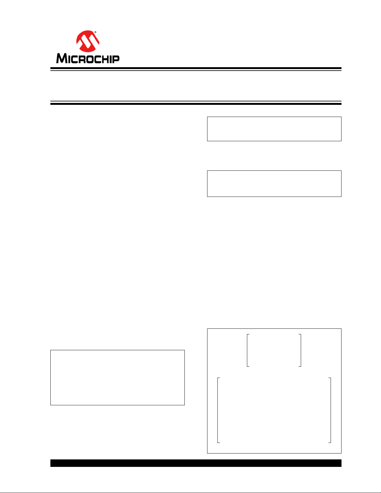
Figure 1 (A) represents the
16 pixels in an image with a 4 x 4 grid. Figure 1 (B)
represents the 64 pixels in an image with an 8 x 8 grid.
Each of the pixels in
Figure 1 (A) is interpolated in 2D
to obtain four pixels in Figure 1 (B). This is the nearest
neighbor interpolation. Since this is a linear interpola-
tion technique, this has the least computation cost. This
technique assumes high correlation in spatial locality of
the same image with different resolutions.
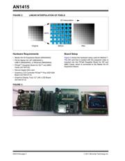
Figure 2
shows the visual representation of the linear
interpolation technique.
FIGURE 1: MATRIX OF ORIGINAL
PIXELS (A) AND
INTERPOLATED PIXELS (B)
BPS HRES VRES FPS BPP⋅⋅⋅=
Where,
BPS = bits per second
H
RES = Horizontal resolution
V
RES = Vertical resolution
FPS = Frames per second
BPP = bits per pixel
BPS 320 240 30 16 36.8Mbps=⋅⋅⋅⋅=
BPS
320
2
-------- -
⎝⎠
⎛⎞
240
2
-------- -
⎝⎠
⎛⎞
30 16 9.2Mbps=⋅⋅⋅=
(A)
(B)
1234
5678
9 10 11 12
13 14 15 16
11223344
11223344
55667788
55667788
9 9 10 10 11 11 12 12
9 9 10 10 11 11 12 12
13 13 14 14 15 15 16 16
13 13 14 14 15 15 16 16
Video Playback and Streaming Solutions
Using the PIC
®
MCU